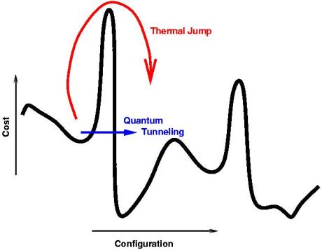
Probabilistic search heuristics such as simulated annealing (SA) are very useful when the search space is extremely large or when the search landscape is non-convex such that basic hill climbing algorithms will tend to get stuck in a local minima.
Whilst SA works well for a variety of problems which are non-convex, quantum annealing can prove to be better for problems where the search landscape is extremely jagged with high variance of values. As SA depends on the temperature of the system to determine transition probabilities to a worse solution, this can be problematic for search spaces where there may be extreme variance in energy between neighboring inputs.
A good example of such a problem is in finding the value of D in minimal solutions of X for which the largest X is generated as a solution to Pell’s equation (specialised quadratic Diophantine equations for which c = 1 in this case). To give an example of the jaggedness of the energy landscape for maximising X, consider the minimal X solution for D equal to 61 and 62. For D = 61, X = 1766319049, while for D = 62, X is only 63. This extremely large variance would even prove troublesome for SA’s transition probabilities function. The key benefit of quantum annealing is that its transition probability function also factors in the width of hill in addition to its height. If the hill is thin enough (in this case it is), the idea is that simulated quantum fluctuations could bring the system out of a shallow local minima.
Below is a barebones implementation in Python for finding the maximum X in minimal solutions for D ≤ 1000. Further improvements could be made to the annealing schedule or adapting the field strength decay rate with respect to the number of iterations run.
import math
import numpy as np
import time

""" Energy Function """

def compute_energy(D):
	""" Takes continued fractions representation of D for integer solutions """
	m = 0
	d = 1
	a_0 = math.floor(D ** 0.5)
	a = a_0
	p_n_1 = 1
	p_n = a_0
	q_n_1 = 0
	q_n = 1
	period = 0
	""" Period finding for continued fraction representation of D"""
	while a != 2 * a_0:
		m = d * a - m
		d = (D - m * m) / d
		a = math.floor((a_0 + m) / d)
		# Recurrence relation for computing convergents
		p_n_2, p_n_1 = p_n_1, p_n
		q_n_2, q_n_1 = q_n_1, q_n
		p_n = a * p_n_1 + p_n_2
		q_n = a * q_n_1 + q_n_2
		period += 1
	""" If period - 1 is odd, then return p_n_1, else iterate period - 1 more times """
	if (period - 1) % 2 == 1:
		return -p_n_1
	elif (period - 1) % 2 == 0:
		if period - 1 == 0:
			return -p_n
		else:
			for _ in xrange(period - 1):
				m = d * a - m
				d = (D - m * m) / d
				a = math.floor((a_0 + m) / d)
				p_n_2, p_n_1 = p_n_1, p_n
				q_n_2, q_n_1 = q_n_1, q_n
				p_n = a * p_n_1 + p_n_2
				q_n = a * q_n_1 + q_n_2
			return -p_n

""" Quantum Annealing """

def quantum_annealing(start_field_strength, field_strength_decay, width, search_space, max_iter):
	start_time = time.time()
	initial_D = search_space[np.random.randint(1, len(search_space))]
	initial_energy = compute_energy(initial_D)
	iter = 0
	while iter < max_iter:
		new_D = search_space[np.random.randint(1, len(search_space))]
		new_energy = compute_energy(new_D)
		if new_energy < initial_energy:
			initial_energy = new_energy
			initial_D = new_D
			start_field_strength *= (1 - field_strength_decay)
		elif new_energy == initial_energy:
			start_field_strength = start_field_strength * (1 - field_strength_decay / 5)
		elif new_energy > initial_energy:
			if np.exp(-((new_energy - initial_energy) ** 0.5) * width / start_field_strength) > np.random.random():
				initial_energy = new_energy
				initial_D = new_D
				start_field_strength *= (1 - field_strength_decay)
			else:
				start_field_strength = start_field_strength * (1 - field_strength_decay / 5)
		iter += 1
	return initial_D, time.time() - start_time

print "Running quantum annealing "

D_list = range(2, 1001)
D_squared = [x ** 2 for x in range(2, 32)]
D_list = [x for x in D_list if x not in D_squared]

counter = 1
while counter < 250:
	print quantum_annealing(100, 0.05, 5, D_list, 1500)
	counter += 1

